Mostafa Firoozi Arani
In business terminology, Cross-selling refers to offering other products or services to customers who are purchasing for another product or service. Although an offer suggestion will not be a great cost for a company, good detection of the potential customers can reduce the chance of reduction of interest of a customer due to spam advertisements, and will make the company able to focus more on the potential customers.
In this project, our aim is to detect potential vehicle insurance buyers, bet`
ween those of whom applied for a health insurance service. There is available a dat
aset with 102351 records, with the columns indicating the data related to each indi
vidual client, as depicted in the table 1. The “Target” attribute indicates that if the s
ubject has been interested in the offer or not.
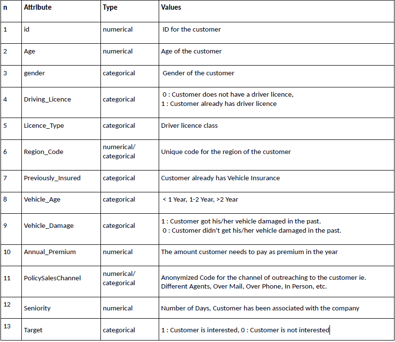
Table 1 Indication of each column data.
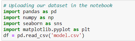
In this phase we investigate our data in terms of homogeneity, existence of null values, etc. We split the data into categorical and numerical and we will work on it. Firstly, we load our dataset in our program after importing the necessary Librar ies. Till now, the required libs are pandas, seaborn, numpy and mathplotlib.
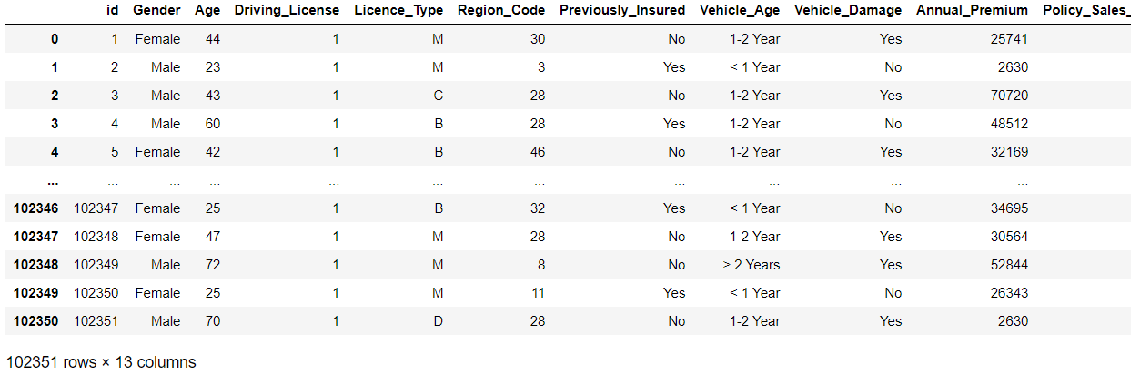
Then, a quick glance at our dataset:
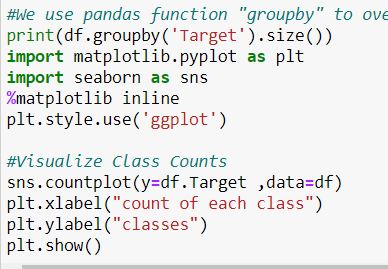
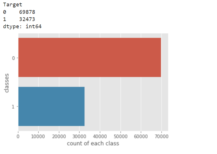
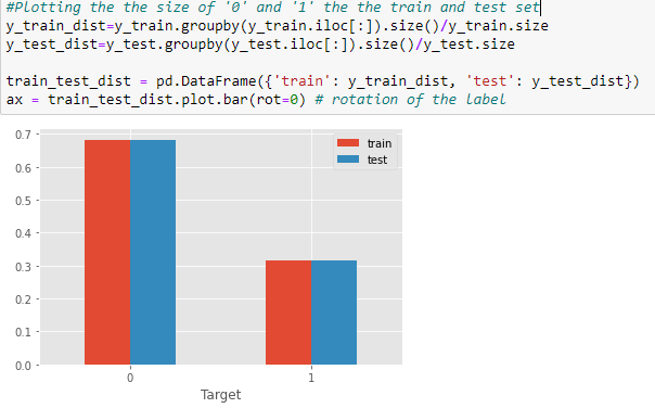
Now, we visualize the how the data is distributed between ‘ 1 ’ and’ 0 ’. Since the gap is not too much, we do not need to down sample the data.
We use df.info function to study all the info about this dataset. As the belo w image represents, we can see Data types, Non-Null values. There are some null values in the column “Licence_Type”, which we need to work on.
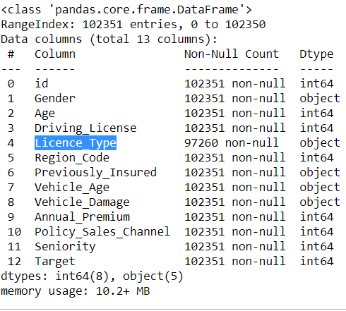
Using the function” df.isna().sum()”, it is illustrated that there are 5091 null values in that column.

We attribute to all the null values in that column, a specific value, “N”, to be able to monitories the values, aiming to opt for eliminating these ‘null’ values or not.

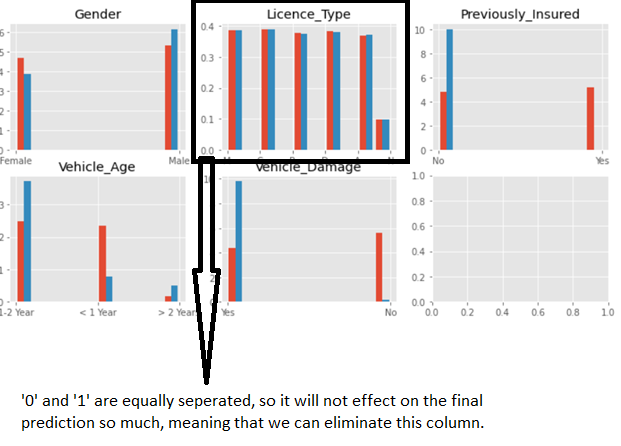
Now we plot the distribution of all the categorical data between ‘ 0 ’ and’ 1’. We see in the all licence_Types the values are equally separated between ‘ 0 ’ and ‘ 1 ’, manifesting that it does not have any serious effect on the final prediction. So we can eliminate all the column, with no worry about corruption of the prediction procedure.

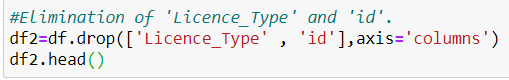
We also drop the column ‘id’, since it does not have any statistical value for us.
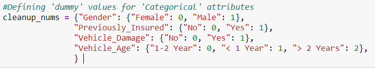
Now we need to define ‘dummy’ values for ‘Categorical’ attributes, to make them applicable in our ML algorithms.
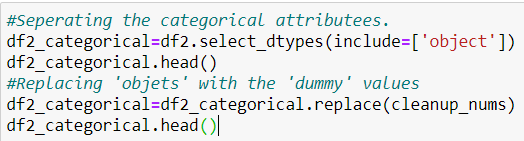
And, Replacing 'objects' with the 'dummy' values.
The very first step with the ‘Numerical’ attributes is to plot the histogram to see its distribution. The below picture represents that, there is a sharp decrease in the ‘Annual_Premium’ attribute. So it would be reasonable the get a logarithm from it using the below code.
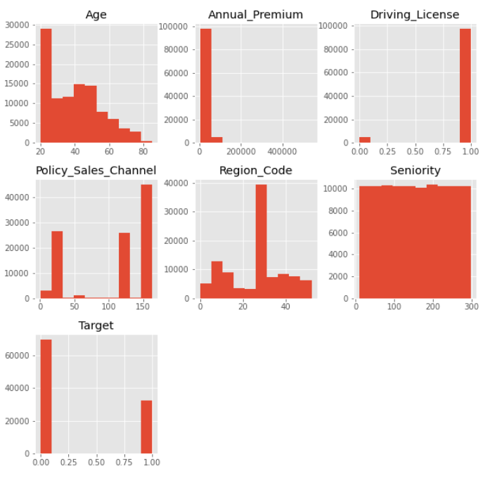
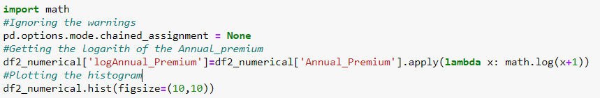
We can see in the new histogram that ‘logAnnual_premium’ has a distribution
more similar to normal.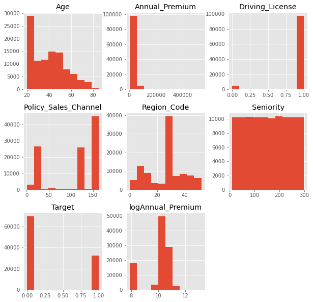
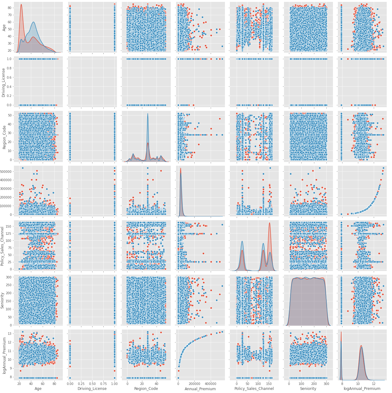
To see how each two ‘Numerical’ attributes distribute in the ‘Target’ value have, we can pair plot all of them a figure. We see the ‘Annual_Premium’ and the ‘log_annual_premium’ have a logarithmic shape relation with each other.
For instance, ‘seniority’ has ‘ gaussian’ distribution, but this distribution is quite the same for ‘ 0 ’ and ‘ 1 ’ which is not a good point. On the other hand, age has two different distribution between ‘ 0 ’ and ‘ 1 ’, make it a more worthy parameter for our prediction.
Now, we will eliminate the ‘Annual_Premium’, since we will be working on ‘logAnnual_Premium’.
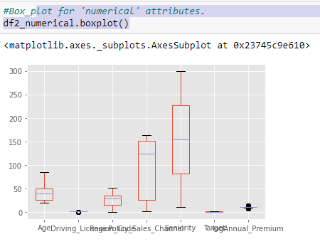
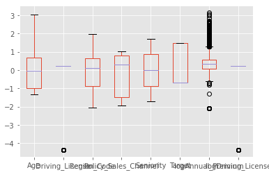
Now, we can boxplot the ‘numerical’ attributes to make a comparison between the different distributions.

Since we have got distributions so deviated from each others, so we should scale the data to receive similar distributions.
We define a scaler, feeding the function with our numerical attributes. We will use this scaler to operate on the other data which we will be using in the future to predict.
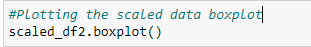
Our scaled dataset will have distributions of the same order for all the ‘numerical’ attributs all arouns ‘ 0 ’.
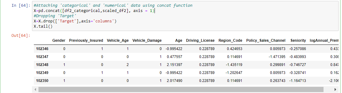
Now we should attach the numerical and categorical attributes, using concat function. Then dropping ‘Target’, since we want to predict the ‘Target’, not using itfor prediction.
Now our dataset is clear, and ready to work on!!!
We define y as the ‘Target’ Values. Then we seperate train and test parts, considering a 70% to 30% division. We stratify our data, to get the same seperation of ‘ 0 ’ and ‘ 1 ’ both in the train and test set.
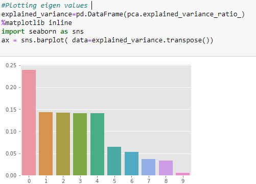
Now we can apply PCA to the data, to check whether we can see a sharp decrease in the data or not. Unfortunately, there is not, so, applying PCA to this dataset is not a good idea.
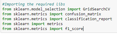
After all these investigations and data preparations, now we can apply our models to our dataset. First off, we import the necessary libraries.
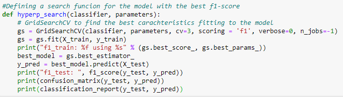
Now we define a function to evaluate the given model with the specified parameters to find out the best parameters fitting the model. We will compare different approaches based on f1-score.
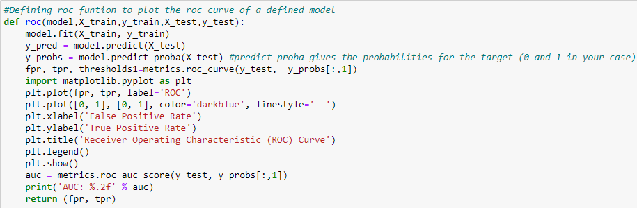
Besides, we define another function to plot ROC curve of a specific model, and calculate the area under that curve.
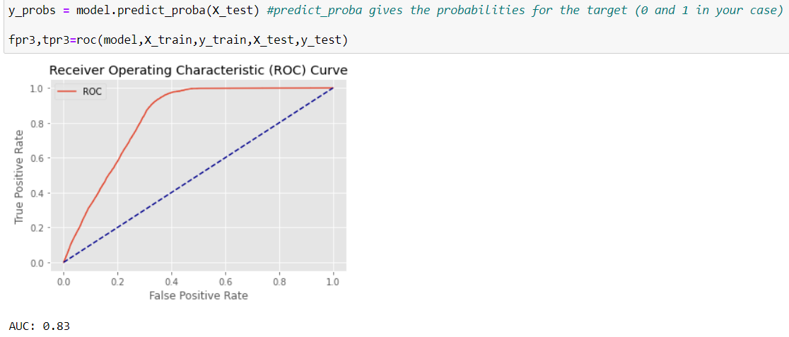
The very first model based on which we want to evaluate is the KNN model. We import this classifier from sklearn.neighbors library. Then, we define 10 different number of neighbors starting from 10, increasing with 100 steps till 1000. Now we can use our hyper_search function to evaluate this classifier through all this set of parameters. According to our function, the best f-score will be achieved using 110 number of neighbors.

Then, we plot the ROC curve of the classifier basing on the defined number.
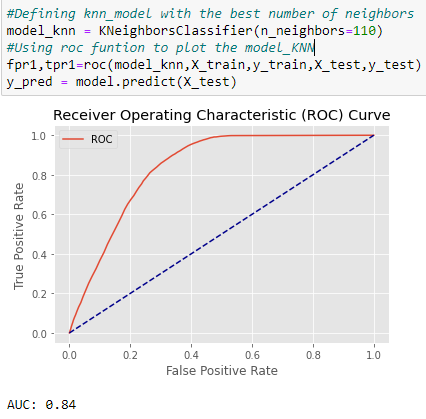
Although an AUC=084 represents a good behaviuor of the model, we will try other models to find the best one.
But the resoult of NaiveBase is less promissing, both based on AUC and f 1 - score.

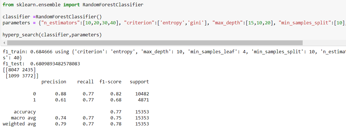
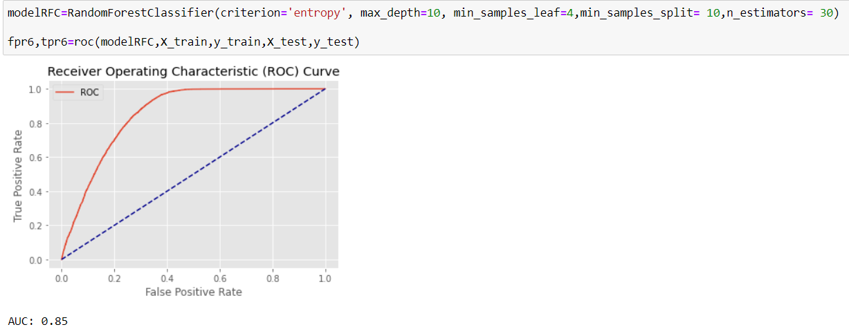
It seems the best result will be achieved using RandonForrestClassifier, both in terms of f1-score and AUC.
Using the offered parameters, we can receive this ROC curve.
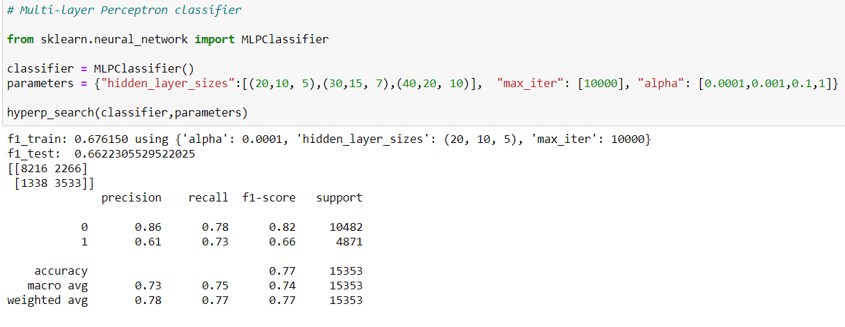
We try the Neural-network classifier as well, with 2 different neural architectures, and 4 different learning rates. After trying the best calculated model, we receive ROC curve quite similar to random forest, but since the f1-score in the random forest is better, our final decision would be that.

After all, we use all the data to train the model since we do not anymore need to evaluate the data
